Clustering Theory

Clustering is the most common form of unsupervised learning. It is the process that involves the grouping of data points into classes of similar objects.

No supervision means that there is no human expert who has assigned labels to the data points. This is a difference from classification.

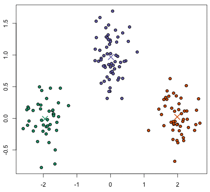
Given a set of data points, we can use a clustering algorithm to classify each data point into a specific group. In theory, data points that are in the same group should have similar properties and/or features, while data points in different groups should have highly dissimilar properties and/or features. A simple example is next figure. It is visually clear that there are three distinct clusters of points.

In Data Science, we can use clustering analysis to gain some valuable insights from our data by observing what groups the data points fall into when we apply a clustering algorithm.

The key input to a clustering algorithm is the distance measure.

Flat clustering creates a flat set of clusters without any explicit structure that would relate clusters to each other. Hierarchical clustering creates a hierarchy of clusters.

K-Means Clustering

K-means is the most important flat clustering algorithm and overall the most well-known clustering algorithm.

Its objective is to minimize the average squared Euclidean distance of the data points from their cluster centers where a cluster center is defined as the mean or centroid. So, the points have to be represented into vectors. The ideal cluster in K-means is a sphere with the centroid as its center of gravity. Ideally, the clusters should not overlap.

A measure of how well the centroids represent the members of their clusters is the residual sum of squares (RSS), the squared distance of each vector from its centroid summed over all vectors K-Means steps:

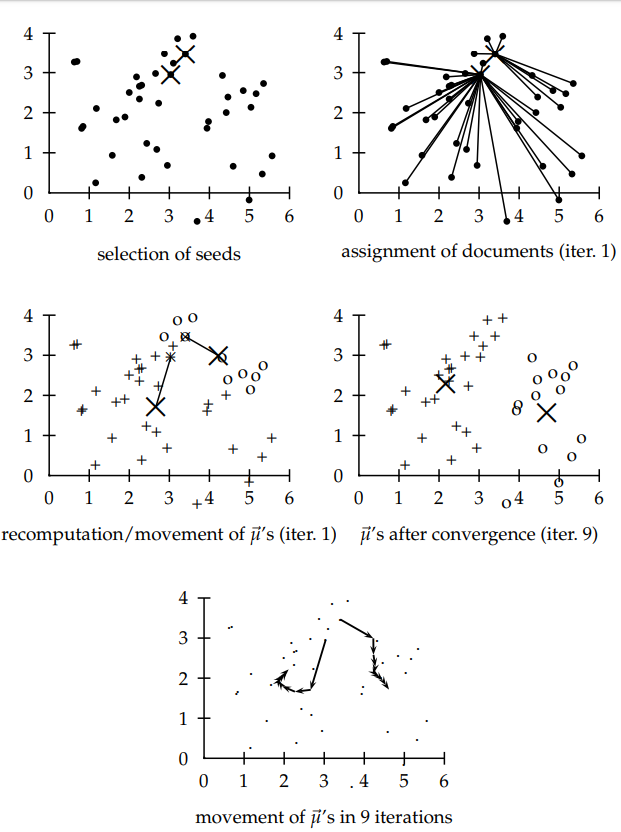
1. We have to select the number of classes that we expect to find and randomly select that many points as centroids. To figure out the number of classes to use, it’s good to take a quick look at the data and try to identify any distinct groupings.
2. Each data point is classified by computing the distance between that point and each group center, and then classifying the point to be in the group whose center is closest to it.
3. Based on these classified points, we recompute the centroids by taking the mean of all the data points in the group.
4. Repeat until the centroids change less than a threshold.

Hyper-parameters

• Number of clusters: The number of clusters and centroids to generate.
• Maximum iterations: Of the algorithm for a single run.
• Number initial: The number of times the algorithm will be run with different centroid seeds. The final result will be the best output of the number defined of consecutives runs, in terms of inertia.

K-Means has the advantage that it’s pretty fast, as all we’re really doing is computing the distances between points and group centers; very few computations! It thus has a linear complexity \(O(n)\).

On the other hand, K-Means has a couple of disadvantages. Firstly, you have to select how many groups/classes there are. This isn’t always trivial and ideally with a clustering algorithm we’d want it to figure those out for us because the point of it is to gain some insight from the data. K-means also starts with a random choice of cluster centers and therefore it may yield different clustering results on different runs of the algorithm. Thus, the results may not be repeatable and lack consistency. Other cluster methods are more consistent.

In order to find the best number of cluster to initialize the algorithm is to estimate \(RSS_min\) as follows:

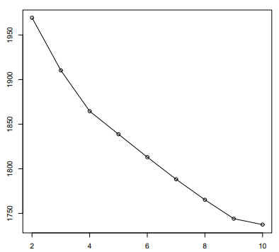
1. We first perform \(i\) (e.g., \(i=10\)) clusterings with K clusters (each with a different initialization) and compute the RSS of each.
2. We take the minimum of the \(i\) RSS values.
3. Inspect the values of \(RSS_min\) as K increases and find the knee in the curve. In the previous figure, the knee in for K=9.

Hierarchical Clustering

It outputs a hierarchy, a structure that is more informative than the unstructured set of clusters returned by flat clustering. It does not require us to pre-specify the number of clusters. These advantages of hierarchical clustering come at the cost of lower efficiency. The most common hierarchical clustering algorithms have a complexity that is at least quadratic in the number of points.

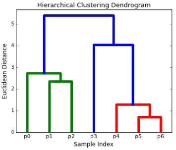
Hierarchical clustering algorithms actually fall into 2 categories: top-down or bottom-up. Bottom-up algorithms treat each data point as a single cluster at the outset and then successively merge (or agglomerate) pairs of clusters until all clusters have been merged into a single cluster that contains all data points. Bottom-up hierarchical clustering is therefore called hierarchical agglomerative clustering. This hierarchy of clusters is represented as a tree (or dendrogram). The root of the tree is the unique cluster that gathers all the samples, the leaves being the clusters with only one sample.

Steps for Agglomerative Hierarchical Clustering:

1. We begin by treating each data point as a single cluster i.e if there are X data points in our dataset then we have X clusters. We then select a distance metric that measures the distance between two clusters. As an example we will use average linkage which defines the distance between two clusters to be the average distance between data points in the first cluster and data points in the second cluster.
2. On each iteration we combine two clusters into one. The two clusters to be combined are selected as those with the smallest average linkage for example. I.e according to our selected distance metric, these two clusters have the smallest distance between each other and therefore are the most similar and should be combined.
3. Step 2 is repeated until we reach the root of the tree. In the end we can select how many clusters we want by choosing when to stop combining.

Linkages to combine clusters

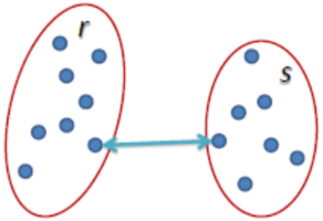
Single Linkage: The distance between two clusters is defined as the shortest distance between two points in each cluster.

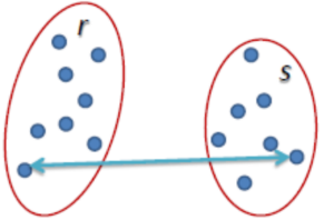
Complete Linkage: The distance between two clusters is defined as the longest distance between two points in each cluster.

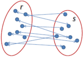
Average Linkage: Τhe distance between two clusters is defined as the average distance between each point in one cluster to every point in the other cluster.

The advantages of hierarchical clustering is that the resulting hierarchical representations can be very informative, and they are especially powerful when the dataset contains real hierarchical relationships.

The disadvantages of hierarchical clustering is that they are very sensitive to outliers and, in their presence, the model performance decreases significantly. They are also very computationally expensive.

Density-Based Spatial Clustering of Applications with Noise (DBSCAN)

DBSCAN is a density based clustered algorithm especially useful to correctly identify noise in data.

Steps for DBSCAN:

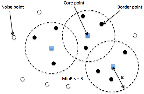
1. DBSCAN begins with an arbitrary starting data point that has not been visited. The neighborhood of this point is extracted using a distance epsilon ε (All points which are within the ε distance are neighborhood points).
2. If there are a sufficient number of points (according to minPoints) within this neighborhood then the clustering process starts and the current data point becomes the first point in the new cluster. Otherwise, the point will be labeled as noise (later this noisy point might become the part of the cluster). In both cases that point is marked as “visited”.
3. For this first point in the new cluster, the points within its ε distance neighborhood also become part of the same cluster. This procedure of making all points in the ε neighborhood belong to the same cluster is then repeated for all of the new points that have been just added to the cluster group.
4. This process of steps 2 and 3 is repeated until all points in the cluster are determined i.e all points within the ε neighborhood of the cluster have been visited and labelled.
5. Once we’re done with the current cluster, a new unvisited point is retrieved and processed, leading to the discovery of a further cluster or noise. This process repeats until all points are marked as visited. Since at the end of this all points have been visited, each point well have been marked as either belonging to a cluster or being noise.

The advantages of DBSCAN is that it does not require a pre-set number of clusters at all. It also identifies outliers as noises unlike mean-shift which simply throws them into a cluster even if the data point is very different. Additionally, it is able to find arbitrarily sized and arbitrarily shaped clusters quite well.

The disadvantage of DBSCAN is that it does not perform as well as others when the clusters are of varying density. This is because the setting of the distance threshold ε and minPoints for identifying the neighborhood points will vary from cluster to cluster when the density varies.